
In a previous post, we learnt to use the OpenAI Gym library to initialise a training environment and to implement a very simple decision policy (either random or hard-coded). I would recommend that you first go through the first post before reading this one. In this post, we will learn a more sophisticated decision-making algorithm : Q-Learning.
Q-learning
Q-Learning is a reinforcement learning (RL) algorithm which seeks to find the best action the agent should take given the current state. The goal is to identify a policy that maximises the expected cumulative reward. Q-learning is:
- model-free : it does not build a representation or model of the environment.
- off-policy : the actions taken by the agent are not (always) guided by the policy that is being learnt. i.e. sometimes the agent follows random actions.
- a temporal difference algorithm: the policy is updated after each time step / action taken.
- value-based : it assigns a Q-value for each action being in a given state.
In its most simple form, Q learning uses a Q-table that store the Q-values of all state-action pairs possible. It updates this table using the Bellman equation. The actions are selected by an \(\epsilon\)-greedy policy. Let’s illustrate these concepts using a simple toy example.
Q-learning by hand
Let’s consider the following problem. The agent (in green) is placed in a 4x4 grid-world environment or maze. Its initial position is in the top-left corner and the goal is to escape the maze by moving to the bottom left corner. The agent has no preliminary knowledge of the environment or the goal to achieve. At each time step, it can perform 4 possible actions: up, down, left or right (unless it is on the edge of the maze). After performing an action, it receives a positive or a negative reward indicated by a score in each cell. There are 16 possible states, shown by a red number. The Q-table is composed of 16 rows (one for each state) and 4 columns (one for each action). For the sake of simplicity, we will initialise the Q-table with zeros, although in practice you’ll want to initialise it with random numbers.
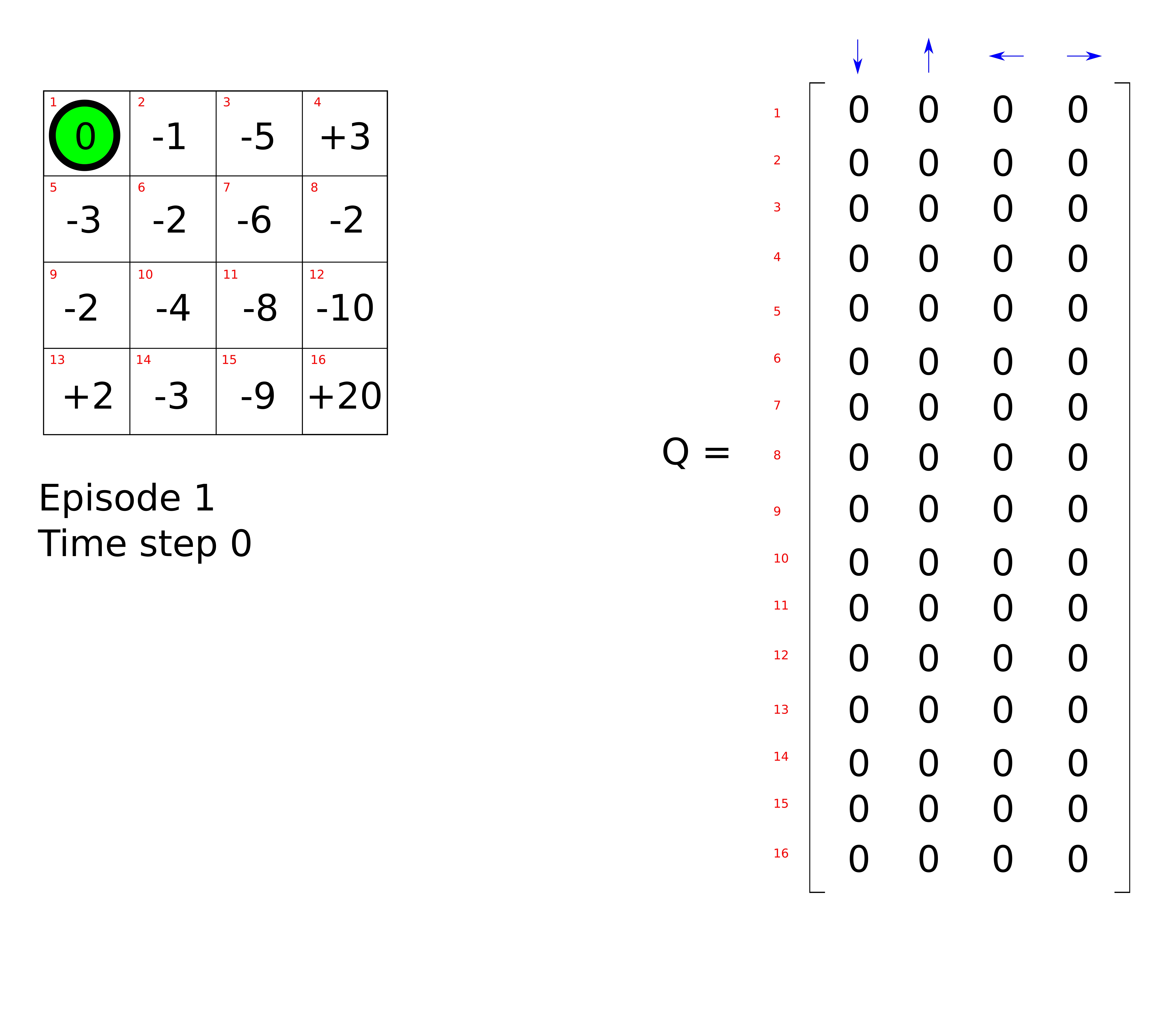
The agent takes an initial random action, for example ‘move right’.
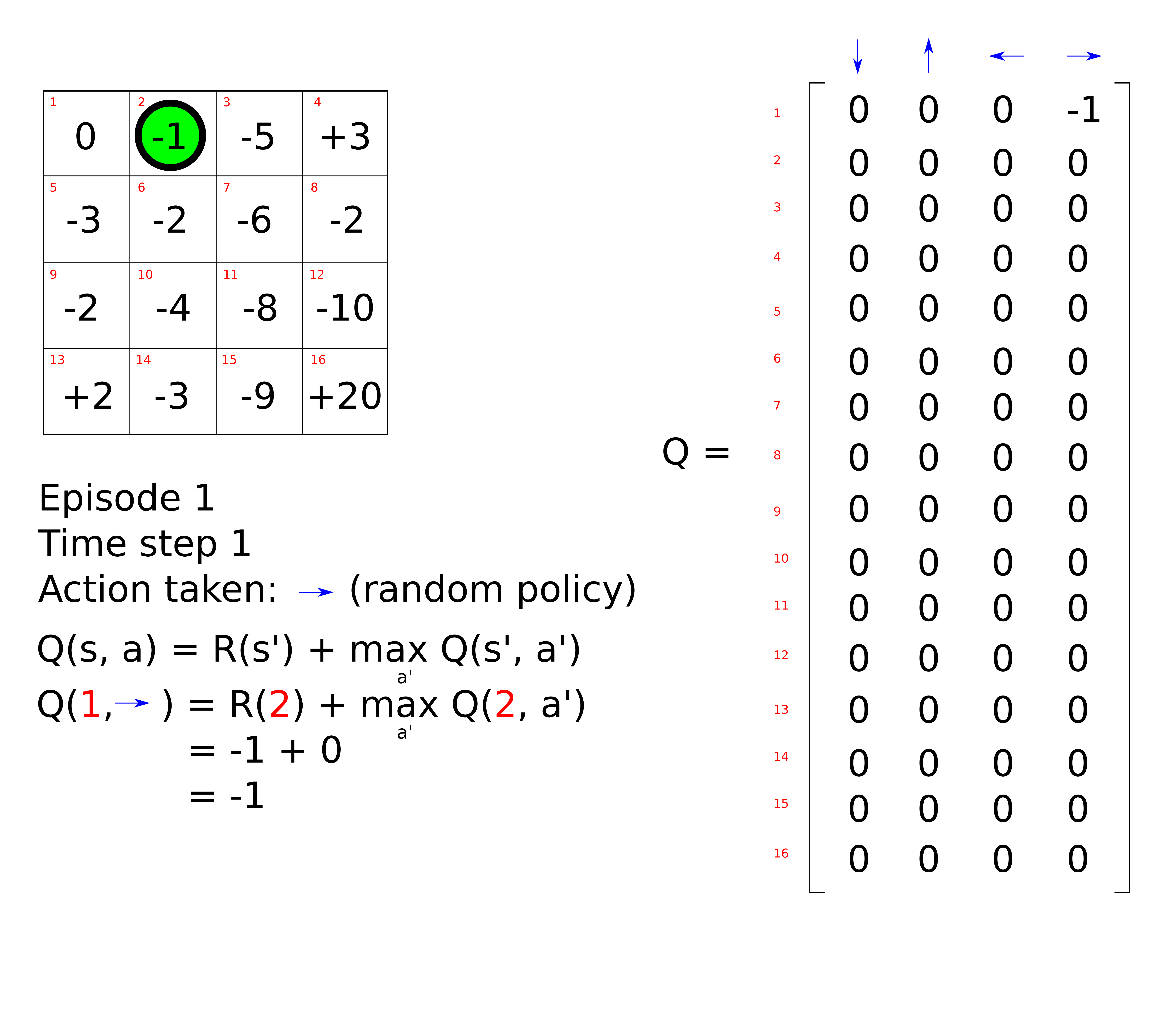
The Q-value associated with being in the initial state (state 1) and moving right is updated using the Bellman equation. In its simplest form, the Bellman equation is written as follows,
\[Q(s, a) = R(s, a) + \gamma \max_{a'} Q(s', a')\]Where
- \(Q(s, a)\) is the Q value of being in state \(s\) and choosing the action \(a\).
- \(R(s, a)\) is the reward obtained from being in state \(s\) and performing action \(a\).
- \(\gamma\) is the discount factor.
- \(\smash{\displaystyle\max_{a'}} \thinspace Q(s', a')\) is the maximum value of all possible future actions \(a'\) being in the next state \(s'\).
The Q value (Q is for “quality”) represents how useful a given action is in gaining some future reward. This equation states that the Q-value yielded from being in a given state and performing a given action is the immediate reward plus the highest Q-value possible from the next state.
The discount factor controls the contribution of rewards further in the future. \(Q(s', a)\) again depends on \(Q(s", a)\) multiplied by a squared discount factor (so the reward at time step t+2 is attenuated compared to the immediate reward at t+1). Each Q-value depends on Q-values of future states as shown here:
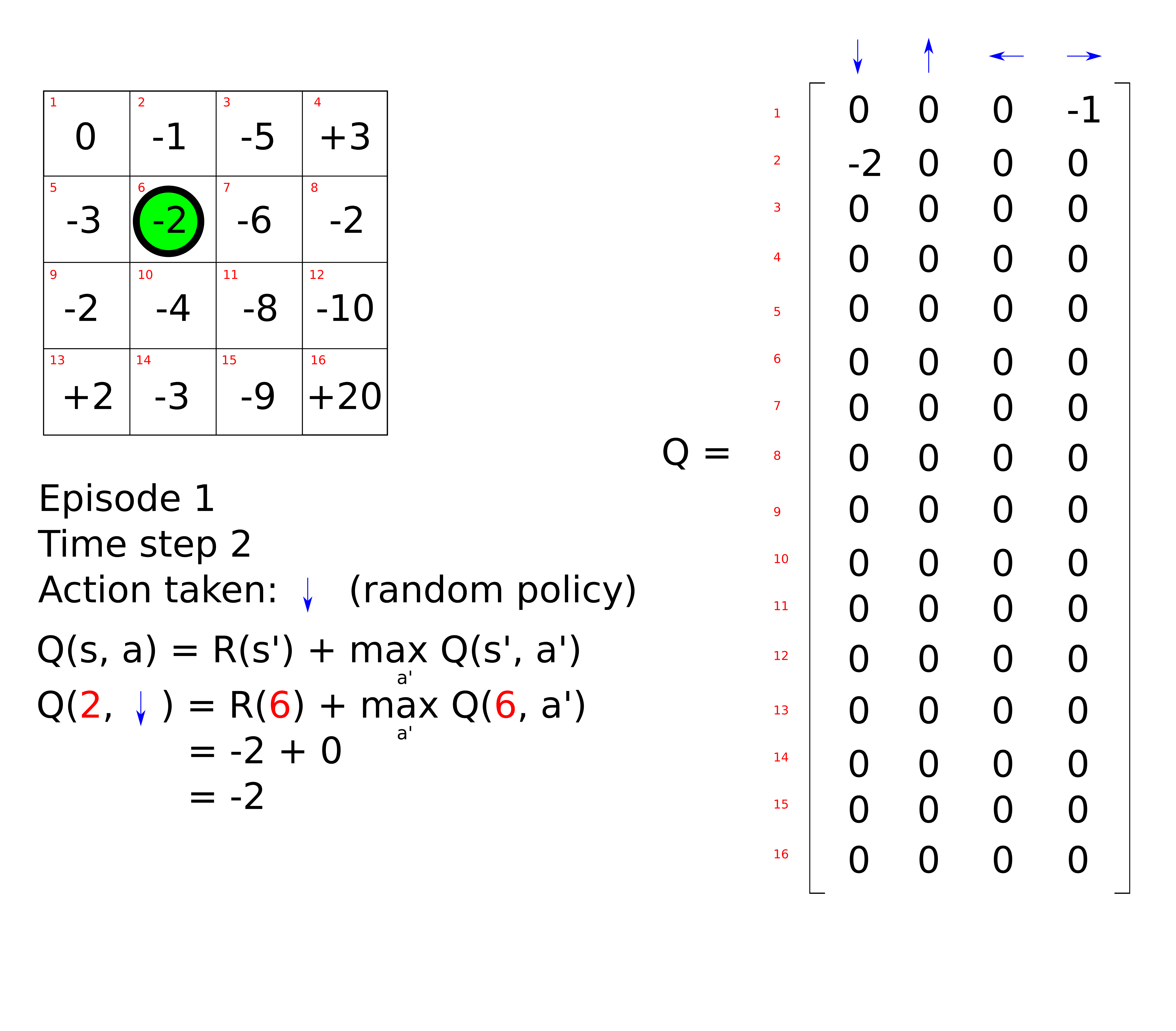
\[Q(s, a) = \gamma Q(s', a') + \gamma^2 Q(s'', a') + ... + \gamma^n Q(s'^{...n}, a')\]In our maze problem, if we assume a discount factor equal to 1, the Q value of being in state 0 and performing action ‘right’ is equal to -1. We can repeat this process by letting the agent take another random action, for example ‘down’. The Q-table is updated as follows.
Here is an animation to illustrate the whole process.
Exploration vs exploitation
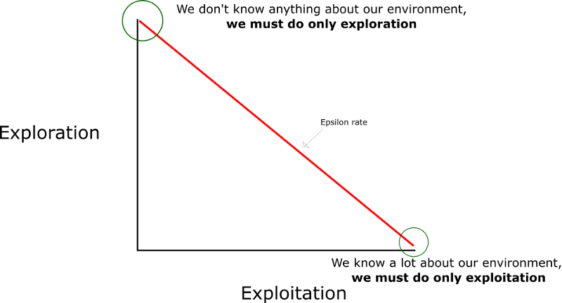
So far, we let the agent explore the environment by taking random actions i.e. it is following a random policy. However, after some time exploring, the agent should capitalise on its past experience by selecting the action that is believed to yield the highest expected reward. This is referred to as exploitation i.e. the agent follows a greedy policy. In order to learn efficiently, there is a trade-off decision to be made between exploration and exploitation. This is implemented in practice by a so-called \(\epsilon\)-greedy policy. At each time step, a number \(\epsilon\) is assigned a value between 0 and 1. Another random number is also selected. If that number is larger than \(\epsilon\), a greedy-action is selected and if it is lower, a random action is chosen. Generally, \(\epsilon\) is decreased from 1 to 0 at each time step during the episode. The decay can be linear as shown below but not necessarily.
This process is repeated iteratively as follows.
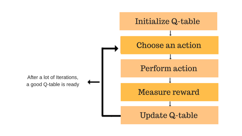
Eventually, the Q-values should converge to a steady values. The training is completed when the squared loss between the predicted and actual Q value is minimal.
\[Loss = (Q(s, a) - \hat{Q}(s, a))^2\]Note: a more sophisticated Bellman equation also include the learning rate as shown below.
\[Q(s, a) = Q(s, a) + \alpha [ R(s, a) + \gamma \max_{a'} Q(s', a') - Q(s, a)]\]If \(\alpha = 0\), the Q value is not updated and if \(\alpha = 1\), we obtain the previous Bellman equation. The learning rate determines to what extent newly acquired information overrides old information.
Let’s see some code – the taxi problem
Let apply Q learning to a benchmark problem from the OpenAI Gym library: the Taxi-v3 environment. The taxi problem consists of a 5-by-5 grid world where a taxi can move. The goal is to pick up a passenger at one of the 4 possible locations and to drop him off in another.
The rules
There are 4 designated locations on the grid that are indicated by a letter: R(ed), B(lue), G(reen), and Y(ellow). When the episode starts, the taxi starts off at a random square and the passenger is at a random location. The taxi drive to the passenger’s location, pick up the passenger, drive to the passenger’s destination (another one of the four specified locations), and then drop off the passenger. Once the passenger is dropped off, the episode ends. You receive +20 points for a successful dropoff, and lose 1 point for every timestep it takes. There is also a 10 point penalty for illegal pick-up and drop-off actions.
There are 500 discrete states since there are 25 taxi positions, 5 possible locations of the passenger (including the case when the passenger is in the taxi), and 4 destination locations. (500 = 25 * 5 * 4).
There are 6 discrete deterministic actions:
- 0: move down
- 1: move up
- 2: move to the right
- 3: move to the left
- 4: pick up a passenger
- 5: drop-off a passenger
The color coding is as follows:
- blue: passenger
- magenta: destination
- yellow: empty taxi
- green: full taxi
- other letters: locations
The code
The code can be found here.
We first initialise the environment.
env = gym.make("Taxi-v3")
We then define some training hyperparameters.
train_episodes = 2000         # Total train episodes
test_episodes = 10            # Total test episodes
n_steps = 100                 # Max steps per episode
alpha = 0.7                   # Learning rate
gamma = 0.618                 # Discounting rate
max_epsilon = 1               # Exploration probability at start
min_epsilon = 0.01            # Minimum exploration probability
decay_rate = 0.01             # Exponential decay rate for exploration prob
We define the greedy and epsilon policies as follows,
def greedy_policy(state):
    return np.argmax(Q[state, :])

def epsilon_policy(state, epsilon):
    exp_exp_tradeoff = random.uniform(0, 1)
    if exp_exp_tradeoff <= epsilon:
        action = env.action_space.sample()  # exploration
    else:
        action = np.argmax(Q[state, :])     # exploitation
    return action
The exploration rate \(\epsilon\) is decreased at each new episode as we require less exploration and more exploitation.
def get_epsilon(episode):
    return min_epsilon + (max_epsilon - min_epsilon) * np.exp(-decay_rate * episode)
The Q table is updated using the Bellman equation as follows,
def update_q(current_state, action, reward, new_state, alpha):
    Q[current_state][action] += alpha * (reward + gamma * np.max(Q[new_state]) - Q[current_state][action])
The training phase is implemented as follow,
training_rewards = []

for episode in range(train_episodes):
    state = env.reset()
    episode_rewards = 0

    epsilon = get_epsilon(episode)

    for t in range(n_steps):
        action = epsilon_policy(state, epsilon)
        new_state, reward, done, info = env.step(action)
        update_q(state, action, reward, new_state, alpha)
        episode_rewards += reward
        state = new_state         # Update the state

        if done:
            print('Episode:{}/{} finished after {} timesteps | Total reward: {}'.format(episode, train_episodes, t+1, episode_rewards))
            break

    training_rewards.append(episode_rewards)

mean_train_reward = sum(training_rewards) / len(training_rewards)
print ("Average cumulated rewards over {} episodes: {}".format(train_episodes, mean_train_reward))
And finally, the agent is tested on the environment:
test_rewards = []

for episode in range(test_episodes):
    state = env.reset()
    episode_rewards = 0

    for t in range(n_steps):
        env.render()
        action = greedy_policy(state)
        new_state, reward, done, info = env.step(action)
        episode_rewards += reward
        state = new_state

        if done:
            print('Episode:{}/{} finished after {} timesteps | Total reward: {}'.format(episode, test_episodes, t+1, episode_rewards))
            break

    test_rewards.append(episode_rewards)

mean_test_reward = sum(test_rewards) / len(test_rewards)
print ("Average cumulated rewards over {} episodes: {}".format(test_episodes, mean_test_reward))
The cumulative reward vs the number of episode is shown below.
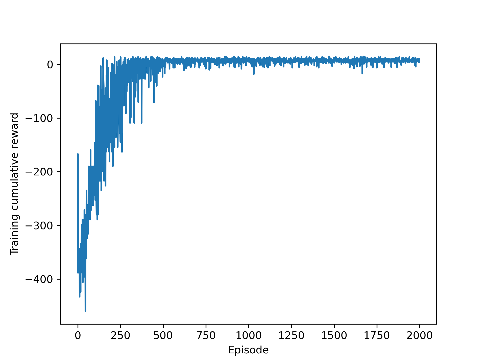
Here is the trained taxi agent in action.
Conclusion
Q-learning is one of the simplest Reinforcement Learning algorithms. One of the main limitation of Q learning is that it can only be applied to problems with a finite number of states such as the maze or the taxi example. For environments with a continuous state space - such as the cart-pole problem - it is no longer possible to define a Q table (else it would need an infinite number of rows). It is possible to discretise the state space into buckets in order to solve this limitation, which I will explain in the next article.


Leave a comment